Vector spherical harmonics

In mathematics, vector spherical harmonics (VSH) are an extension of the scalar spherical harmonics for use with vector fields. The components of the VSH are complex-valued functions expressed in the spherical coordinate basis vectors.

DefinitionEdit

Several conventions have been used to define the VSH.^{[1][2][3][4][5]} We follow that of Barrera et al.. Given a scalar spherical harmonic Y_lm(θ, φ), we define three VSH:

• ${\displaystyle \mathbf {Y} _{lm}=Y_{lm}{\hat {\mathbf {r} }},}$
• ${\displaystyle \mathbf {\Psi } _{lm}=r\nabla Y_{lm},}$
• ${\displaystyle \mathbf {\Phi } _{lm}=\mathbf {r} \times \nabla Y_{lm},}$

with ${\displaystyle {\hat {\mathbf {r} }}}$ being the unit vector along the radial direction in spherical coordinates and ${\displaystyle \mathbf {r} }$ the vector along the radial direction with the same norm as the radius, i.e., ${\displaystyle \mathbf {r} =r{\hat {\mathbf {r} }}}$. The radial factors are included to guarantee that the dimensions of the VSH are the same as those of the ordinary spherical harmonics and that the VSH do not depend on the radial spherical coordinate.

The interest of these new vector fields is to separate the radial dependence from the angular one when using spherical coordinates, so that a vector field admits a multipole expansion

${\displaystyle \mathbf {E} =\sum _{l=0}^{\infty }\sum _{m=-l}^{l}\left(E_{lm}^{r}(r)\mathbf {Y} _{lm}+E_{lm}^{(1)}(r)\mathbf {\Psi } _{lm}+E_{lm}^{(2)}(r)\mathbf {\Phi } _{lm}\right).}$

The labels on the components reflect that ${\displaystyle E_{lm}^{r}}$ is the radial component of the vector field, while ${\displaystyle E_{lm}^{(1)}}$ and ${\displaystyle E_{lm}^{(2)}}$ are transverse components (with respect to the radius vector ${\displaystyle \mathbf {r} }$).

Main PropertiesEdit

SymmetryEdit

Like the scalar spherical harmonics, the VSH satisfy

${\displaystyle {\begin{aligned}\mathbf {Y} _{l,-m}&=(-1)^{m}\mathbf {Y} _{lm}^{*},\\\mathbf {\Psi } _{l,-m}&=(-1)^{m}\mathbf {\Psi } _{lm}^{*},\\\mathbf {\Phi } _{l,-m}&=(-1)^{m}\mathbf {\Phi } _{lm}^{*},\end{aligned}}}$

which cuts the number of independent functions roughly in half. The star indicates complex conjugation.

OrthogonalityEdit

The VSH are orthogonal in the usual three-dimensional way at each point ${\displaystyle \mathbf {r} }$:

${\displaystyle {\begin{aligned}\mathbf {Y} _{lm}(\mathbf {r} )\cdot \mathbf {\Psi } _{lm}(\mathbf {r} )&=0,\\\mathbf {Y} _{lm}(\mathbf {r} )\cdot \mathbf {\Phi } _{lm}(\mathbf {r} )&=0,\\\mathbf {\Psi } _{lm}(\mathbf {r} )\cdot \mathbf {\Phi } _{lm}(\mathbf {r} )&=0.\end{aligned}}}$

They are also orthogonal in Hilbert space:

${\displaystyle {\begin{aligned}\int \mathbf {Y} _{lm}\cdot \mathbf {Y} _{l'm'}^{*}\,d\Omega &=\delta _{ll'}\delta _{mm'},\\\int \mathbf {\Psi } _{lm}\cdot \mathbf {\Psi } _{l'm'}^{*}\,d\Omega &=l(l+1)\delta _{ll'}\delta _{mm'},\\\int \mathbf {\Phi } _{lm}\cdot \mathbf {\Phi } _{l'm'}^{*}\,d\Omega &=l(l+1)\delta _{ll'}\delta _{mm'},\\\int \mathbf {Y} _{lm}\cdot \mathbf {\Psi } _{l'm'}^{*}\,d\Omega &=0,\\\int \mathbf {Y} _{lm}\cdot \mathbf {\Phi } _{l'm'}^{*}\,d\Omega &=0,\\\int \mathbf {\Psi } _{lm}\cdot \mathbf {\Phi } _{l'm'}^{*}\,d\Omega &=0.\end{aligned}}}$

An additional result at a single point ${\displaystyle \mathbf {r} }$ (not reported in Barrera et al, 1985) is, for all ${\displaystyle l,m,l',m'}$,

${\displaystyle {\begin{aligned}\mathbf {Y} _{lm}(\mathbf {r} )\cdot \mathbf {\Psi } _{l'm'}(\mathbf {r} )&=0,\\\mathbf {Y} _{lm}(\mathbf {r} )\cdot \mathbf {\Phi } _{l'm'}(\mathbf {r} )&=0.\end{aligned}}}$

Vector multipole momentsEdit

The orthogonality relations allow one to compute the spherical multipole moments of a vector field as

${\displaystyle {\begin{aligned}E_{lm}^{r}&=\int \mathbf {E} \cdot \mathbf {Y} _{lm}^{*}\,d\Omega ,\\E_{lm}^{(1)}&={\frac {1}{l(l+1)}}\int \mathbf {E} \cdot \mathbf {\Psi } _{lm}^{*}\,d\Omega ,\\E_{lm}^{(2)}&={\frac {1}{l(l+1)}}\int \mathbf {E} \cdot \mathbf {\Phi } _{lm}^{*}\,d\Omega .\end{aligned}}}$

The gradient of a scalar fieldEdit

Given the multipole expansion of a scalar field

${\displaystyle \phi =\sum _{l=0}^{\infty }\sum _{m=-l}^{l}\phi _{lm}(r)Y_{lm}(\theta ,\phi ),}$

we can express its gradient in terms of the VSH as

${\displaystyle \nabla \phi =\sum _{l=0}^{\infty }\sum _{m=-l}^{l}\left({\frac {d\phi _{lm}}{dr}}\mathbf {Y} _{lm}+{\frac {\phi _{lm}}{r}}\mathbf {\Psi } _{lm}\right).}$

DivergenceEdit

For any multipole field we have

${\displaystyle {\begin{aligned}\nabla \cdot \left(f(r)\mathbf {Y} _{lm}\right)&=\left({\frac {df}{dr}}+{\frac {2}{r}}f\right)Y_{lm},\\\nabla \cdot \left(f(r)\mathbf {\Psi } _{lm}\right)&=-{\frac {l(l+1)}{r}}fY_{lm},\\\nabla \cdot \left(f(r)\mathbf {\Phi } _{lm}\right)&=0.\end{aligned}}}$

By superposition we obtain the divergence of any vector field:

${\displaystyle \nabla \cdot \mathbf {E} =\sum _{l=0}^{\infty }\sum _{m=-l}^{l}\left({\frac {dE_{lm}^{r}}{dr}}+{\frac {2}{r}}E_{lm}^{r}-{\frac {l(l+1)}{r}}E_{lm}^{(1)}\right)Y_{lm}.}$

We see that the component on Φ_lm is always solenoidal.

CurlEdit

For any multipole field we have

${\displaystyle {\begin{aligned}\nabla \times \left(f(r)\mathbf {Y} _{lm}\right)&=-{\frac {1}{r}}f\mathbf {\Phi } _{lm},\\\nabla \times \left(f(r)\mathbf {\Psi } _{lm}\right)&=\left({\frac {df}{dr}}+{\frac {1}{r}}f\right)\mathbf {\Phi } _{lm},\\\nabla \times \left(f(r)\mathbf {\Phi } _{lm}\right)&=-{\frac {l(l+1)}{r}}f\mathbf {Y} _{lm}-\left({\frac {df}{dr}}+{\frac {1}{r}}f\right)\mathbf {\Psi } _{lm}.\end{aligned}}}$

By superposition we obtain the curl of any vector field:

${\displaystyle \nabla \times \mathbf {E} =\sum _{l=0}^{\infty }\sum _{m=-l}^{l}\left(-{\frac {l(l+1)}{r}}E_{lm}^{(2)}\mathbf {Y} _{lm}-\left({\frac {dE_{lm}^{(2)}}{dr}}+{\frac {1}{r}}E_{lm}^{(2)}\right)\mathbf {\Psi } _{lm}+\left(-{\frac {1}{r}}E_{lm}^{r}+{\frac {dE_{lm}^{(1)}}{dr}}+{\frac {1}{r}}E_{lm}^{(1)}\right)\mathbf {\Phi } _{lm}\right).}$

LaplacianEdit

The action of the Laplace operator ${\displaystyle \Delta =\nabla \cdot \nabla }$ separates as follows:

${\displaystyle \Delta \left(f(r)\mathbf {Z} _{lm}\right)=\left({\frac {1}{r^{2}}}{\frac {\partial }{\partial r}}r^{2}{\frac {\partial f}{\partial r}}\right)\mathbf {Z} _{lm}+f(r)\Delta \mathbf {Z} _{lm},}$

where ${\displaystyle \mathbf {Z} _{lm}=\mathbf {Y} _{lm},\mathbf {\Psi } _{lm},\mathbf {\Phi } _{lm}}$ and

${\displaystyle {\begin{aligned}\Delta \mathbf {Y} _{lm}&=-{\frac {1}{r^{2}}}(2+l(l+1))\mathbf {Y} _{lm}+{\frac {2}{r^{2}}}\mathbf {\Psi } _{lm},\\\Delta \mathbf {\Psi } _{lm}&={\frac {2}{r^{2}}}l(l+1)\mathbf {Y} _{lm}-{\frac {1}{r^{2}}}l(l+1)\mathbf {\Psi } _{lm},\\\Delta \mathbf {\Phi } _{lm}&=-{\frac {1}{r^{2}}}l(l+1)\mathbf {\Phi } _{lm}.\end{aligned}}}$

Also note that this action becomes symmetric, i.e. the off-diagonal coefficients are equal to ${\displaystyle {\frac {2}{r^{2}}}{\sqrt {l(l+1)}}}$, for properly normalized VSH.

ExamplesEdit

First vector spherical harmonicsEdit

• ${\displaystyle l=0}$.

${\displaystyle {\begin{aligned}\mathbf {Y} _{00}&={\sqrt {\frac {1}{4\pi }}}{\hat {\mathbf {r} }},\\\mathbf {\Psi } _{00}&=\mathbf {0} ,\\\mathbf {\Phi } _{00}&=\mathbf {0} .\end{aligned}}}$

• ${\displaystyle l=1}$.

${\displaystyle {\begin{aligned}\mathbf {Y} _{10}&={\sqrt {\frac {3}{4\pi }}}\cos \theta \,{\hat {\mathbf {r} }},\\\mathbf {Y} _{11}&=-{\sqrt {\frac {3}{8\pi }}}e^{i\varphi }\sin \theta \,{\hat {\mathbf {r} }},\end{aligned}}}$

${\displaystyle {\begin{aligned}\mathbf {\Psi } _{10}&=-{\sqrt {\frac {3}{4\pi }}}\sin \theta \,{\hat {\mathbf {\theta } }},\\\mathbf {\Psi } _{11}&=-{\sqrt {\frac {3}{8\pi }}}e^{i\varphi }\left(\cos \theta \,{\hat {\mathbf {\theta } }}+i\,{\hat {\mathbf {\varphi } }}\right),\end{aligned}}}$

${\displaystyle {\begin{aligned}\mathbf {\Phi } _{10}&=-{\sqrt {\frac {3}{4\pi }}}\sin \theta \,{\hat {\mathbf {\varphi } }},\\\mathbf {\Phi } _{11}&={\sqrt {\frac {3}{8\pi }}}e^{i\varphi }\left(i\,{\hat {\mathbf {\theta } }}-\cos \theta \,{\hat {\mathbf {\varphi } }}\right).\end{aligned}}}$

• ${\displaystyle l=2}$.

${\displaystyle {\begin{aligned}\mathbf {Y} _{20}&={\frac {1}{4}}{\sqrt {\frac {5}{\pi }}}\,(3\cos ^{2}\theta -1)\,{\hat {\mathbf {r} }},\\\mathbf {Y} _{21}&=-{\sqrt {\frac {15}{8\pi }}}\,\sin \theta \,\cos \theta \,e^{i\varphi }\,{\hat {\mathbf {r} }},\\\mathbf {Y} _{22}&={\frac {1}{4}}{\sqrt {\frac {15}{2\pi }}}\,\sin ^{2}\theta \,e^{2i\varphi }\,{\hat {\mathbf {r} }}.\end{aligned}}}$

${\displaystyle {\begin{aligned}\mathbf {\Psi } _{20}&=-{\frac {3}{2}}{\sqrt {\frac {5}{\pi }}}\,\sin \theta \,\cos \theta \,{\hat {\mathbf {\theta } }},\\\mathbf {\Psi } _{21}&=-{\sqrt {\frac {15}{8\pi }}}\,e^{i\varphi }\,\left(\cos 2\theta \,{\hat {\mathbf {\theta } }}+i\cos \theta \,{\hat {\mathbf {\varphi } }}\right),\\\mathbf {\Psi } _{22}&={\sqrt {\frac {15}{8\pi }}}\,\sin \theta \,e^{2i\varphi }\,\left(\cos \theta \,{\hat {\mathbf {\theta } }}+i\,{\hat {\mathbf {\varphi } }}\right).\end{aligned}}}$

${\displaystyle {\begin{aligned}\mathbf {\Phi } _{20}&=-{\frac {3}{2}}{\sqrt {\frac {5}{\pi }}}\sin \theta \,\cos \theta \,{\hat {\mathbf {\varphi } }},\\\mathbf {\Phi } _{21}&={\sqrt {\frac {15}{8\pi }}}\,e^{i\varphi }\,\left(i\cos \theta \,{\hat {\mathbf {\theta } }}-\cos 2\theta \,{\hat {\mathbf {\varphi } }}\right),\\\mathbf {\Phi } _{22}&={\sqrt {\frac {15}{8\pi }}}\,\sin \theta \,e^{2i\varphi }\,\left(-i\,{\hat {\mathbf {\theta } }}+\cos \theta \,{\hat {\mathbf {\varphi } }}\right).\end{aligned}}}$

Expressions for negative values of m are obtained by applying the symmetry relations.

ApplicationsEdit

ElectrodynamicsEdit

The VSH are especially useful in the study of multipole radiation fields. For instance, a magnetic multipole is due to an oscillating current with angular frequency ${\displaystyle \omega }$ and complex amplitude

${\displaystyle {\hat {\mathbf {J} }}=J(r)\mathbf {\Phi } _{lm},}$

and the corresponding electric and magnetic fields, can be written as

${\displaystyle {\begin{aligned}{\hat {\mathbf {E} }}&=E(r)\mathbf {\Phi } _{lm},\\{\hat {\mathbf {B} }}&=B^{r}(r)\mathbf {Y} _{lm}+B^{(1)}(r)\mathbf {\Psi } _{lm}.\end{aligned}}}$

Substituting into Maxwell equations, Gauss' law is automatically satisfied

${\displaystyle \nabla \cdot {\hat {\mathbf {E} }}=0,}$

while Faraday's law decouples as

${\displaystyle \nabla \times {\hat {\mathbf {E} }}=-i\omega {\hat {\mathbf {B} }}\quad \Rightarrow \quad \left\{{\begin{array}{l}\displaystyle {\frac {l(l+1)}{r}}E=i\omega B^{r},\\\displaystyle {\frac {dE}{dr}}+{\frac {E}{r}}=i\omega B^{(1)}.\end{array}}\right.}$

Gauss' law for the magnetic field implies

${\displaystyle \nabla \cdot {\hat {\mathbf {B} }}=0\quad \Rightarrow \quad {\frac {dB^{r}}{dr}}+{\frac {2}{r}}B^{r}-{\frac {l(l+1)}{r}}B^{(1)}=0,}$

and Ampère-Maxwell's equation gives

${\displaystyle \nabla \times {\hat {\mathbf {B} }}=\mu _{0}{\hat {\mathbf {J} }}+i\mu _{0}\varepsilon _{0}\omega {\hat {\mathbf {E} }}\quad \Rightarrow \quad -{\frac {B^{r}}{r}}+{\frac {dB^{(1)}}{dr}}+{\frac {B^{(1)}}{r}}=\mu _{0}J+i\omega \mu _{0}\varepsilon _{0}E.}$

In this way, the partial differential equations have been transformed into a set of ordinary differential equations.

Alternative definitionEdit

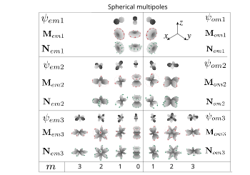
Angular part of magnetic and electric vector spherical harmonics. Red and green arrows show the direction of the field. Generating scalar functions are also presented, only the first three orders are shown (dipoles, quadrupoles, octupoles).

In many applications, vector spherical harmonics are defined as fundamental set of the solutions of vector Helmholtz equation in spherical coordinates.^[6][7]

In this case, vector spherical harmonics are generated by scalar functions, which are solutions of scalar Helmholtz equation with the wavevector ${\displaystyle {\bf {k}}}$.

${\displaystyle {\begin{array}{l}{\psi _{emn}=\cos m\varphi P_{n}^{m}(\cos \vartheta )z_{n}({k}r)}\\{\psi _{omn}=\sin m\varphi P_{n}^{m}(\cos \vartheta )z_{n}({k}r)}\end{array}}}$

here ${\displaystyle P_{n}^{m}(\cos \theta )}$ - associated Legendre polynomials, and ${\displaystyle z_{n}({k}r)}$ - any of spherical Bessel functions.

Vector spherical harmonics are defined as:

${\displaystyle \mathbf {L} _{^{e}_{o}mn}=\mathbf {\nabla } \psi _{^{e}_{o}mn}}$ - longitual harmonics

${\displaystyle \mathbf {M} _{^{e}_{o}mn}=\nabla \times \left(\mathbf {r} \psi _{^{e}_{o}mn}\right)}$ - magnetic harmonics

${\displaystyle \mathbf {N} _{^{e}_{o}mn}={\frac {\nabla \times \mathbf {M} _{^{e}_{o}mn}}{k}}}$ - electric harmonics

Here we use harmonics real-valued angular part, where ${\displaystyle m\geq 0}$, but complex functions can be introduced in the same way .

Let us introduce the notation ${\displaystyle \rho =kr}$. In the component form vector spherical harmonics are written as:

${\displaystyle {\begin{aligned}{\mathbf {M} _{emn}(k,\mathbf {r} )={{\frac {-m}{\sin(\theta )}}\sin(m\varphi )P_{n}^{m}(\cos(\theta ))}z_{n}(\rho )\mathbf {e} _{\theta }-}\\{-\cos(m\varphi ){\frac {dP_{n}^{m}(\cos(\theta ))}{d\theta }}}z_{n}(\rho )\mathbf {e} _{\varphi }\end{aligned}}}$

${\displaystyle {\begin{aligned}{\mathbf {M} _{omn}(k,\mathbf {r} )={{\frac {m}{\sin(\theta )}}\cos(m\varphi )P_{n}^{m}(\cos(\theta ))}}z_{n}(\rho )\mathbf {e} _{\theta }-\\{-\sin(m\varphi ){\frac {dP_{n}^{m}(\cos(\theta ))}{d\theta }}z_{n}(\rho )\mathbf {e} _{\varphi }}\end{aligned}}}$

${\displaystyle {\begin{aligned}{\mathbf {N} _{emn}(k,\mathbf {r} )={\frac {z_{n}(\rho )}{\rho }}\cos(m\varphi )n(n+1)P_{n}^{m}(\cos(\theta ))\mathbf {e} _{\mathbf {r} }+}\\{+\cos(m\varphi ){\frac {dP_{n}^{m}(\cos(\theta ))}{d\theta }}}{\frac {1}{\rho }}{\frac {d}{d\rho }}\left[\rho z_{n}(\rho )\right]\mathbf {e} _{\theta }-\\{-m\sin(m\varphi ){\frac {P_{n}^{m}(\cos(\theta ))}{\sin(\theta )}}}{\frac {1}{\rho }}{\frac {d}{d\rho }}\left[\rho z_{n}(\rho )\right]\mathbf {e} _{\varphi }\end{aligned}}}$

${\displaystyle {\begin{aligned}\mathbf {N} _{omn}&(k,\mathbf {r} )={\frac {z_{n}(\rho )}{\rho }}\sin(m\varphi )n(n+1)P_{n}^{m}(\cos(\theta ))\mathbf {e} _{\mathbf {r} }+\\&+\sin(m\varphi ){\frac {dP_{n}^{m}(\cos(\theta ))}{d\theta }}{\frac {1}{\rho }}{\frac {d}{d\rho }}\left[\rho z_{n}(\rho )\right]\mathbf {e} _{\theta }+\\&+{m\cos(m\varphi ){\frac {P_{n}^{m}(\cos(\theta ))}{\sin(\theta )}}}{\frac {1}{\rho }}{\frac {d}{d\rho }}\left[\rho z_{n}(\rho )\right]\mathbf {e} _{\varphi }\end{aligned}}}$

There is no radial part for magnetic harmonics. For electric harmonics, the radial part decreases faster than angular, and for big ${\displaystyle \rho }$ can be neglected. We can also see that for electric and magnetic harmonics angular parts are the same up to permutation of the polar and azimuthal unit vectors, so for big ${\displaystyle \rho }$ electric and magnetic harmonics vectors are equal in value and perpendicular to each other.

Longitual harmonics:

${\displaystyle {\begin{aligned}\mathbf {L} _{^{e}_{o}{mn}}&(k,\mathbf {r} )={\frac {\partial }{\partial r}}z_{n}(kr)P_{n}^{m}(\cos \theta ){^{\cos }_{\sin }}{m\varphi }\mathbf {e} _{r}+\\&{\frac {1}{r}}z_{n}(kr){\frac {\partial }{\partial \theta }}P_{n}^{m}(\cos \theta ){^{\cos }_{\sin }}m\varphi \mathbf {e} _{\theta }\mp \\&\mp {\frac {m}{r\sin \theta }}z_{n}(kr)P_{n}^{m}(\cos \theta ){^{\sin }_{\cos }}m\varphi \mathbf {e} _{\varphi }\end{aligned}}}$

OrthogonalityEdit

The solutions of the Helmholtz vector equation obey the following orthogonality relations:^[7]

${\displaystyle {\int _{0}^{2\pi }\int _{0}^{\pi }\mathbf {L} _{^{e}_{o}mn}\cdot \mathbf {L} _{^{e}_{o}mn}\sin \vartheta d\vartheta d\varphi }{=(1+\delta _{m,0}){\frac {2\pi }{(2n+1)^{2}}}{\frac {(n+m)!}{(n-m)!}}k^{2}\left\{n\left[z_{n-1}(kr)\right]^{2}+(n+1)\left[z_{n+1}(kr)\right]^{2}\right\}}}$

${\displaystyle {\int _{0}^{2\pi }\int _{0}^{\pi }\mathbf {M} _{^{e}_{o}mn}\cdot \mathbf {M} _{^{e}_{o}mn}\sin \vartheta d\vartheta d\varphi }{=(1+\delta _{m,0}){\frac {2\pi }{2n+1}}{\frac {(n+m)!}{(n-m)!}}n(n+1)\left[z_{n}(kr)\right]^{2}}}$

${\displaystyle \int _{0}^{2\pi }\int _{0}^{\pi }\mathbf {N} _{^{e}_{o}mn}\cdot \mathbf {N} _{^{e}_{o}mn}\sin \vartheta d\vartheta d\varphi }{=(1+\delta _{m,0}){\frac {2\pi }{(2n+1)^{2}}}{\frac {(n+m)!}{(n-m)!}}n(n+1)\left\{(n+1)\left[z_{n-1}(kr)\right]^{2}+n\left[z_{n+1}(kr)\right]^{2}\right\}}$

${\displaystyle {\int _{0}^{\pi }\int _{0}^{2\pi }\mathbf {L} _{^{e}_{o}mn}\cdot \mathbf {N} _{^{e}_{o}mn}\sin \vartheta d\vartheta d\varphi }{=(1+\delta _{m,0}){\frac {2\pi }{(2n+1)^{2}}}{\frac {(n+m)!}{(n-m)!}}n(n+1)k\left\{\left[z_{n-1}(kr)\right]^{2}-\left[z_{n+1}(kr)\right]^{2}\right\}}}$

All other integrals over the angles between different functions or functions with different indices are equal to zero.

Rotation and inversionEdit

Illustration of the transformation of vector spherical harmonics under rotations. One can see that they are transformed in the same way as the corresponding scalar functions.

Under rotation, vector spherical harmonics are transformed through each other in the same way as the corresponding scalar spherical functions, which are generating for a specific type of vector harmonics. For example, if the generating functions are the usual spherical harmonics, then the vector harmonics will also be transformed through the Wigner D-matrixes^[8][9][10]

${\displaystyle {\hat {D}}(\alpha ,\beta ,\gamma )\mathbf {Y} _{JM}^{(s)}(\theta ,\varphi )=\sum _{m'=-\ell }^{\ell }[D_{MM'}^{(\ell )}(\alpha ,\beta ,\gamma )]^{*}\mathbf {Y} _{JM'}^{(s)}(\theta ,\varphi ),}$

The behavior under rotations is the same for electrical, magnetic and longitudinal harmonics.

Under inversion, electric and longitudinal spherical harmonics behave in the same way as scalar spherical functions, i.e.

${\displaystyle {\hat {I}}\mathbf {N} _{JM}(\theta ,\varphi )=(-1)^{J}\mathbf {N} _{JM}(\theta ,\varphi ),}$

and magnetic ones have the opposite parity:

${\displaystyle {\hat {I}}\mathbf {M} _{JM}(\theta ,\varphi )=(-1)^{J+1}\mathbf {M} _{JM}(\theta ,\varphi ),}$

Fluid dynamicsEdit

In the calculation of the Stokes' law for the drag that a viscous fluid exerts on a small spherical particle, the velocity distribution obeys Navier-Stokes equations neglecting inertia, i.e.,

${\displaystyle {\begin{aligned}\nabla \cdot \mathbf {v} &=0,\\\mathbf {0} &=-\nabla p+\eta \nabla ^{2}\mathbf {v} ,\end{aligned}}}$

with the boundary conditions

${\displaystyle {\begin{aligned}\mathbf {v} &=\mathbf {0} \quad (r=a),\\\mathbf {v} &=-\mathbf {U} _{0}\quad (r\to \infty ).\end{aligned}}}$

where U is the relative velocity of the particle to the fluid far from the particle. In spherical coordinates this velocity at infinity can be written as

${\displaystyle \mathbf {U} _{0}=U_{0}\left(\cos \theta \,{\hat {\mathbf {r} }}-\sin \theta \,{\hat {\mathbf {\theta } }}\right)=U_{0}\left(\mathbf {Y} _{10}+\mathbf {\Psi } _{10}\right).}$

The last expression suggests an expansion in spherical harmonics for the liquid velocity and the pressure

${\displaystyle {\begin{aligned}p&=p(r)Y_{10},\\\mathbf {v} &=v^{r}(r)\mathbf {Y} _{10}+v^{(1)}(r)\mathbf {\Psi } _{10}.\end{aligned}}}$ 

Substitution in the Navier–Stokes equations produces a set of ordinary differential equations for the coefficients.

Integral relationsEdit

Here the following definitions are used:

${\displaystyle {\begin{aligned}Y_{emn}&=\cos m\varphi P_{n}^{m}(\cos \theta )\\Y_{omn}&=\sin m\varphi P_{n}^{m}(\cos \theta )\end{aligned}}}$

${\displaystyle \mathbf {X} _{^{e}_{o}mn}\left({\frac {\mathbf {k} }{k}}\right)=\nabla \times \left(\mathbf {k} Y_{^{o}_{e}mn}\left({\frac {\mathbf {k} }{k}}\right)\right)}$

${\displaystyle \mathbf {Z} _{^{o}_{e}mn}\left({\frac {\mathbf {k} }{k}}\right)=i{\frac {\mathbf {k} }{k}}\times \mathbf {X} _{^{e}_{o}mn}\left({\frac {\mathbf {k} }{k}}\right)}$

In case, when instead of ${\displaystyle z_{n}}$ are spherical bessel functions, with help of plane wave expansion one can obtain the following integral relations:^[11]

${\displaystyle \mathbf {N} _{pmn}(k,\mathbf {r} )={\frac {i^{-n}}{4\pi }}\int \mathbf {Z} _{pmn}\left({\frac {\mathbf {k} }{k}}\right)e^{i\mathbf {k} \mathbf {r} }d\Omega _{k}}$

${\displaystyle \mathbf {M} _{pmn}(k,\mathbf {r} )={\frac {i^{-n}}{4\pi }}\int \mathbf {X} _{pmn}\left({\frac {\mathbf {k} }{k}}\right)e^{i\mathbf {k} \mathbf {r} }d\Omega _{k}}$

In case, when ${\displaystyle z_{n}}$ are spherical hankel functions, one should use the different formulae.^[12][11] For vector spherical harmonics the following relations are obtained:

${\displaystyle \mathbf {M} _{pmn}^{(3)}(k,\mathbf {r} )={\frac {i^{-n}}{2\pi k}}\iint _{-\infty }^{\infty }dk_{\|}{\frac {e^{i\left(k_{x}x+k_{y}y\pm k_{z}z\right)}}{k_{z}}}\left[\mathbf {X} _{pmn}\left({\frac {\mathbf {k} }{k}}\right)\right]}$

${\displaystyle \mathbf {N} _{pmn}^{(3)}(k,\mathbf {r} )={\frac {i^{-n}}{2\pi k}}\iint _{-\infty }^{\infty }dk_{\|}{\frac {e^{i\left(k_{x}x+k_{y}y\pm k_{z}z\right)}}{k_{z}}}\left[\mathbf {Z} _{pmn}\left({\frac {\mathbf {k} }{k}}\right)\right]}$

where , index  means, that spherical hankel functions are used. 

This article uses material from the Wikipedia article  Metasyntactic variable, which is released under the  Creative Commons Attribution-ShareAlike 3.0 Unported License.